Login



MLEP in KICS for Networks 5.0: how machine learning helps track network behavior of OT devices

In an industrial network, malicious activity can be hard to tell apart from normal data exchange between devices. Malicious actors routinely rely on legitimate tools and the Living-off-the-Land technique, so a single network connection may show no known signs of an attack: the device uses a familiar protocol and transmits ordinary data. An anomaly can hide in subtle details: the data source, the time of access, or the volume of transferred data may be atypical for a particular device. However, to detect this kind of anomaly, you need to understand the roles of the devices at both ends of the connection and know which network activity patterns are typical for them.
But an organization’s asset inventory data is often incomplete, which makes it harder to catch unauthorized connections in time. Suppose monitoring detects a host that regularly exchanges data with programmable logic controllers (PLCs). Its IP address is known, but the inventory does not specify what role it plays: is it an engineering workstation, a process data server, or a piece of contractor’s equipment? The host may also have been on the industrial network for a long time, with its record going out of date after a network upgrade.
In the joint OT asset inventory guidance released by CISA and its partners in 2025, inventorying devices and classifying them by role are treated as part of OT asset management. For organizations, this is one of the most important areas: according to the SANS 2025 ICS security survey, 50% of respondents had deployed or significantly expanded ICS inventory and visibility tools over the previous 12 months, and 54% named them as investment priorities for the next 12–24 months.
Device inventory in Kaspersky Industrial CyberSecurity for Networks
In Kaspersky Industrial CyberSecurity for Networks, the Asset Discovery technology is the foundation of asset visibility. Passive network traffic analysis detects devices and their interactions, while recognition rules help determine the device category and extract available information about it, such as the vendor, model, or software version. Exactly which attributes the system can obtain depends on the protocol and the traffic it observes. We covered this in more detail at the Kaspersky Industrial Cybersecurity Conference.
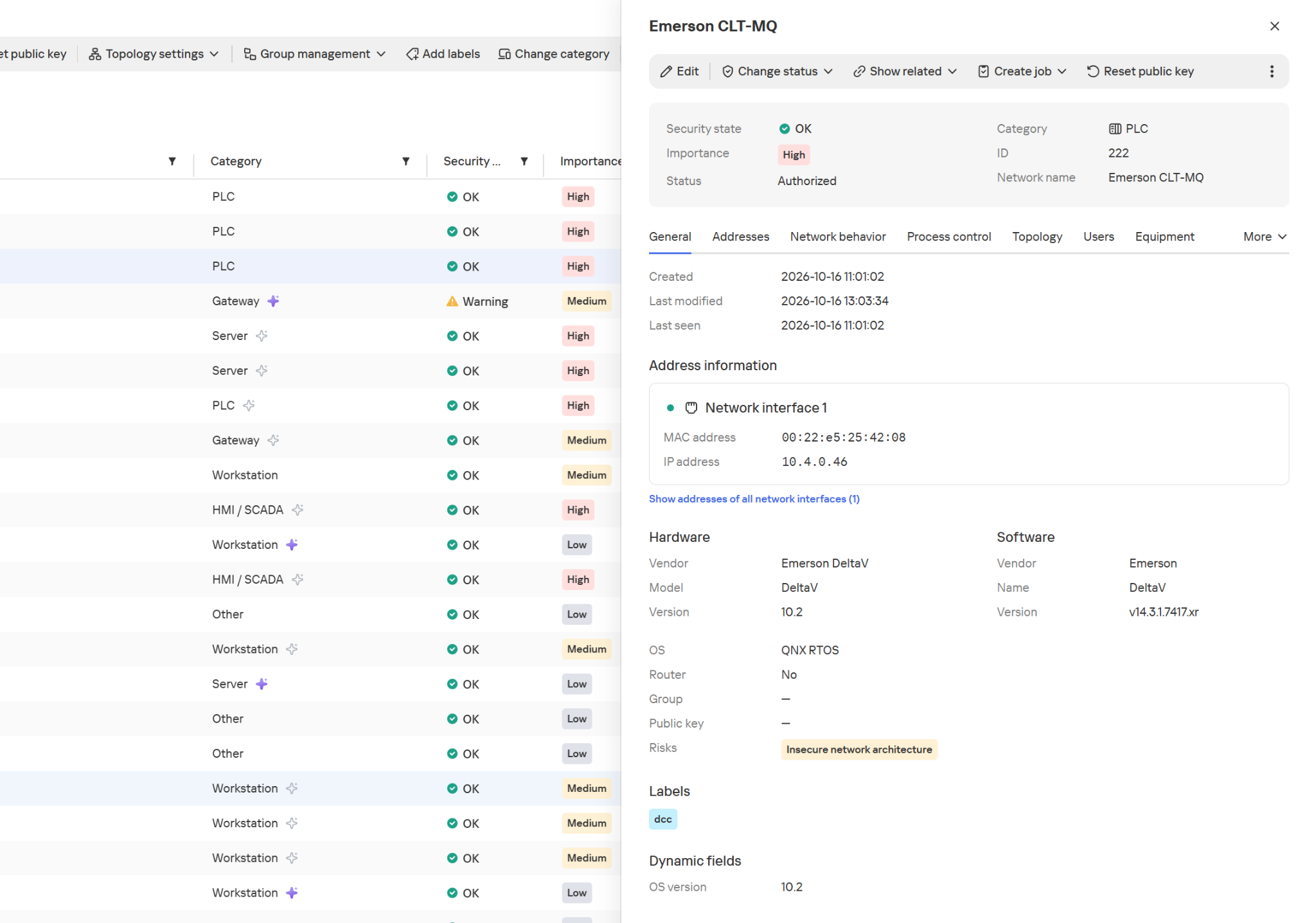
Hardware and software information in the device card
The product also supports active polling modules (APMs): where polling is allowed, they can request additional configuration and firmware version details from devices. This kind of inventory is far more detailed than a list of IP addresses.
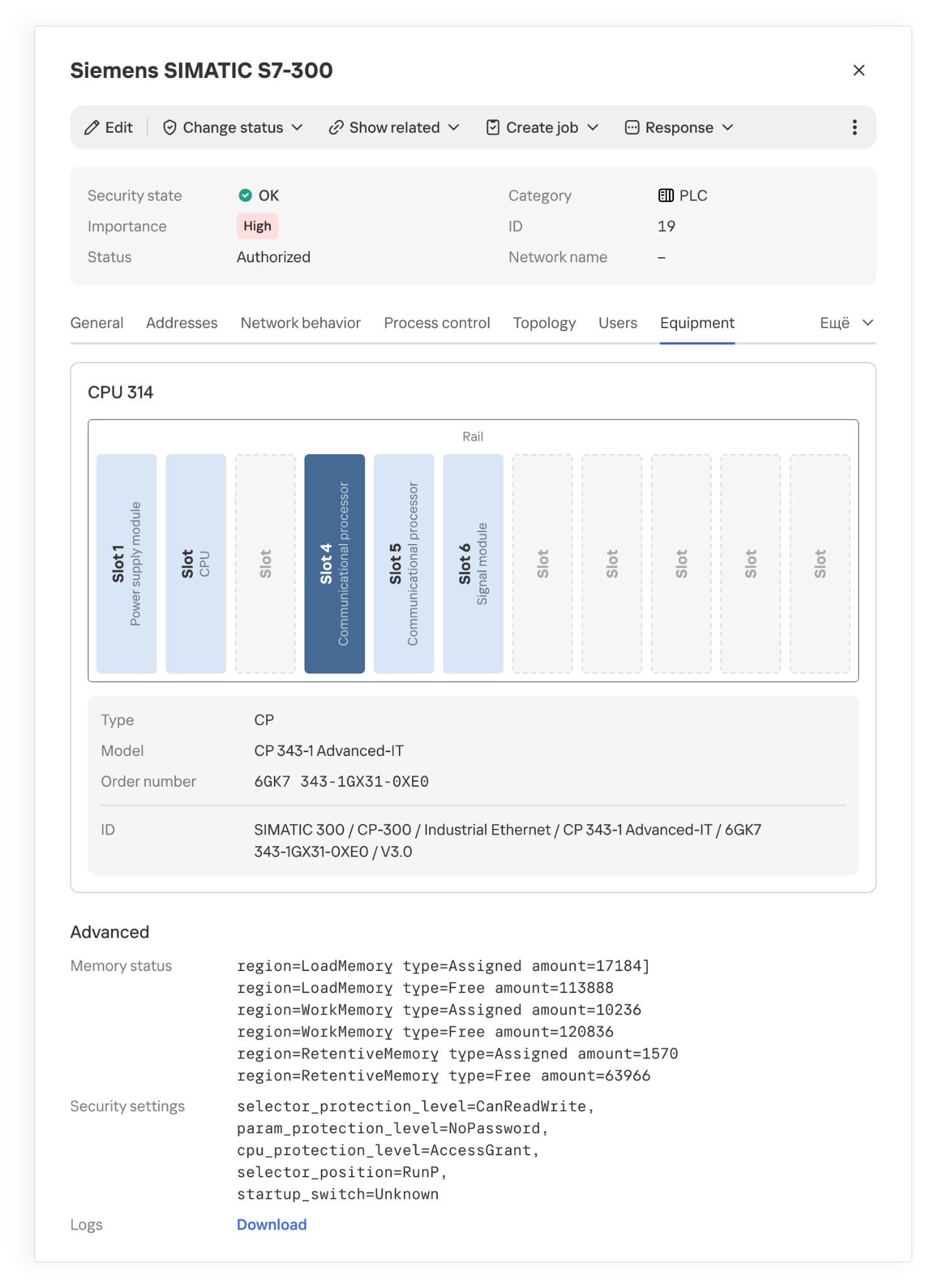
Installed modules and their placement in a PLC rack
However, even accurate hardware information doesn’t always explain what function a host performs in a specific industrial facility. Gaps appear for various reasons. Some devices send identifying information only at startup or during configuration, while others rarely communicate. Proprietary protocols can’t always be parsed, and encryption may leave only connection metadata for analysis. If the monitoring system doesn’t receive traffic from every segment of the industrial network, some network activity goes unobserved. Active polling doesn’t suit every device or every operating condition.
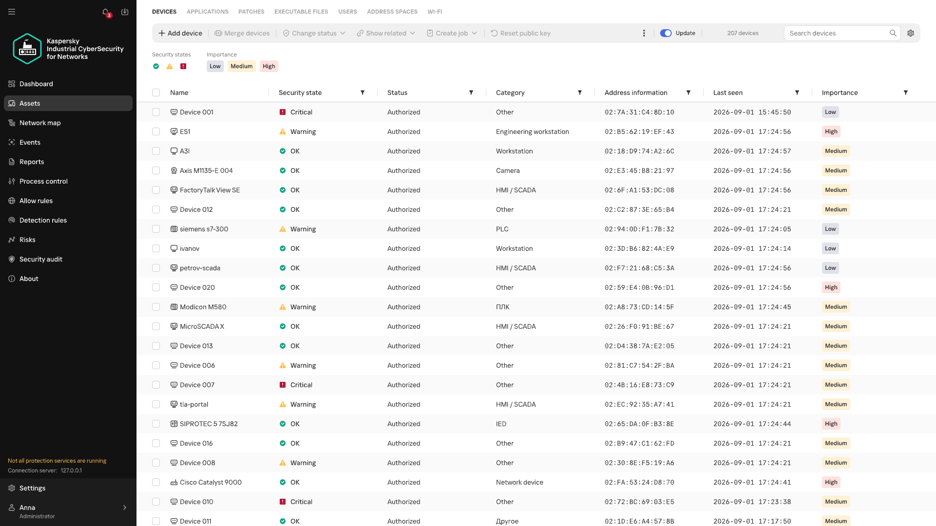
Devices of unknown category
When there isn’t enough direct information about a device, its category can be refined by looking at the patterns of its recurring network interactions. Analyzing these interactions is the job of Machine Learning Event Processor (MLEP), a service included in Kaspersky Industrial CyberSecurity for Networks 5.0. This machine-learning-based event processor can both refine device categories and detect anomalies in their network behavior.
What data does MLEP analyze?
To compare device behavior, you don’t need to store every packet as a separate observation (a data object) in the ML model. MLEP represents network sessions as a sequence of short 15-second fragments. For each fragment, MLEP stores information about the endpoints (IP, MAC, and port), the direction of data exchange, the protocol, and the number and size of the packets transmitted. Together these make up an event, which then gets a timestamp. Traffic thus becomes a sequence of events showing which hosts a device communicated with, when, and how communication intensity changed.
Aggregating data into events also sets the method’s limits. An aggregated fragment can’t be used to reconstruct the exact order of individual packets or the content of commands. MLEP can draw conclusions about a new protocol only if another KICS technology has managed to recognize it. That said, comparing stable network connections and changes in exchange volume doesn’t require a detailed record of every packet. These observations form the basis of the device’s behavioral history.
From observations to MLEP results
Each object has its own behavioral history, and one object’s history can’t be applied to another. But the principles of behavior analysis, along with some common rules, work across different objects.
Let’s look at how this works in MLEP, which is built on a spiking neural semantic network (NSN).
Event identification
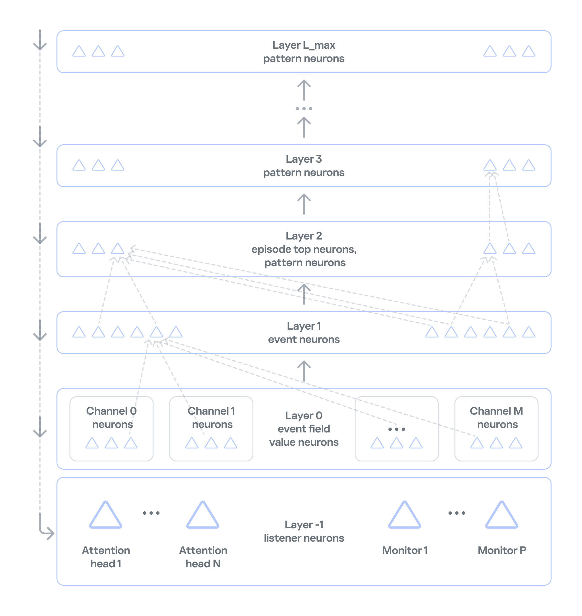
Neurosemantic networks structure information as a multilayer ordered graph, where the data in each consecutive layer builds on the data in the previous one. The nodes of this graph — that is, the units of information in each layer — act as neurons.The NSN creates dedicated channels to handle different event parameters (port, IP, and so on). Unique parameter values for each channel are stored as neurons in layer 0. The event itself, which consists of a set of parameter values, is stored as a neuron in layer 1 of the network. If an event occurs for the first time, neurogenesis creates a new neuron with input connections to the corresponding parameter neurons. This lets the network learn and operate on the event stream at the same time. If the event has occurred before, the network activates the same neuron that was created when the event first appeared. This way, the network identifies each event precisely. Each neuron that corresponds to an event also collects basic statistics: when it was last activated and how many times it has been activated.
Event history
In NSN-based event processing, layer 2 and above store sequences of events over time: recurring patterns and the full history. However, categorization and statistical anomaly detection don’t require storing the full packet sequence or a detailed timeline of every network event. As we noted earlier, events are themselves aggregates, which means the order of network packets has already been averaged out. So MLEP keeps history only temporarily, within each episode (30,000 aggregated events by default), which saves computing resources.
Statistics processing in MLEP
MLEP processes statistics mainly through specialized listener neurons on layer −1 (minus one) of the network. Attention heads and monitors are built on these neurons.
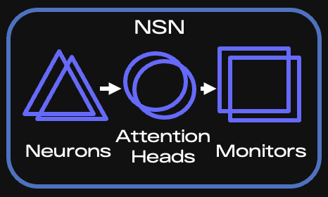
Key components of the NSN
When an event arrives, the corresponding neuron is activated, and the network instantly knows whether that neuron is new or was created earlier. Each attention head subscribes to the events or event features it needs and takes in only the activations of the matching neurons. If an event occurs for the first time, all heads are notified and then decide whether to subscribe (grow a connection to the relevant neuron) and receive information about activations of such neurons from then on.
It is called a spiking network because activation information is a spike, not a number. This spike tells the head that something it’s interested in has happened.
An attention head is configured according to scenarios — the situations that MLEP should send alerts about. The core of a head’s configuration is a query, which filters incoming information and serves as the subscription criterion. Unlike regular database queries, this query runs on the stream, so it can react to an event instantly.
Attention heads work very much like the semantics of ordinary human language. A query has a subject of attention (one or more grammatical subjects) and conditions (the other parts of the sentence). In the infrastructure of an industrial enterprise, the subjects are devices on the network, and the conditions are various aspects of network communication, such as ports, protocol, and average packet size. If a head has many subjects (for example, if it’s interested in every device on an industrial network), it fans out: it creates a child head for each individual value of the subject of attention, that is, each device. The child head then watches a specific device and reports to the parent head.
Attention heads don’t accumulate or process statistics. They only filter event streams. When an attention head receives a relevant event, it activates and sends a spike to the monitor subscribed to that head.
Monitors, in turn, have stacks for accumulating and processing events. They can also have their own queries and post-filter information from the head. For example, they can select only new events from those filtered by the head.
There are several types of monitors:
- Stat monitors track changes in the average count of specific events (for example, device activity) over time intervals typical for those events, or in the average values of numeric event parameters (for example, changes in device traffic volume).
- Monitors work from the event alone: they fire when an event has occurred a certain number of times within a given interval, or has occurred for the first time.
- Similar-behavior monitors work with heads that can generalize events, that is, extract just a few parameters whose combination is shared (generalized) across many events.
MLEP uses these monitor types to implement scenarios for categorizing devices and detecting their anomalous behavior:
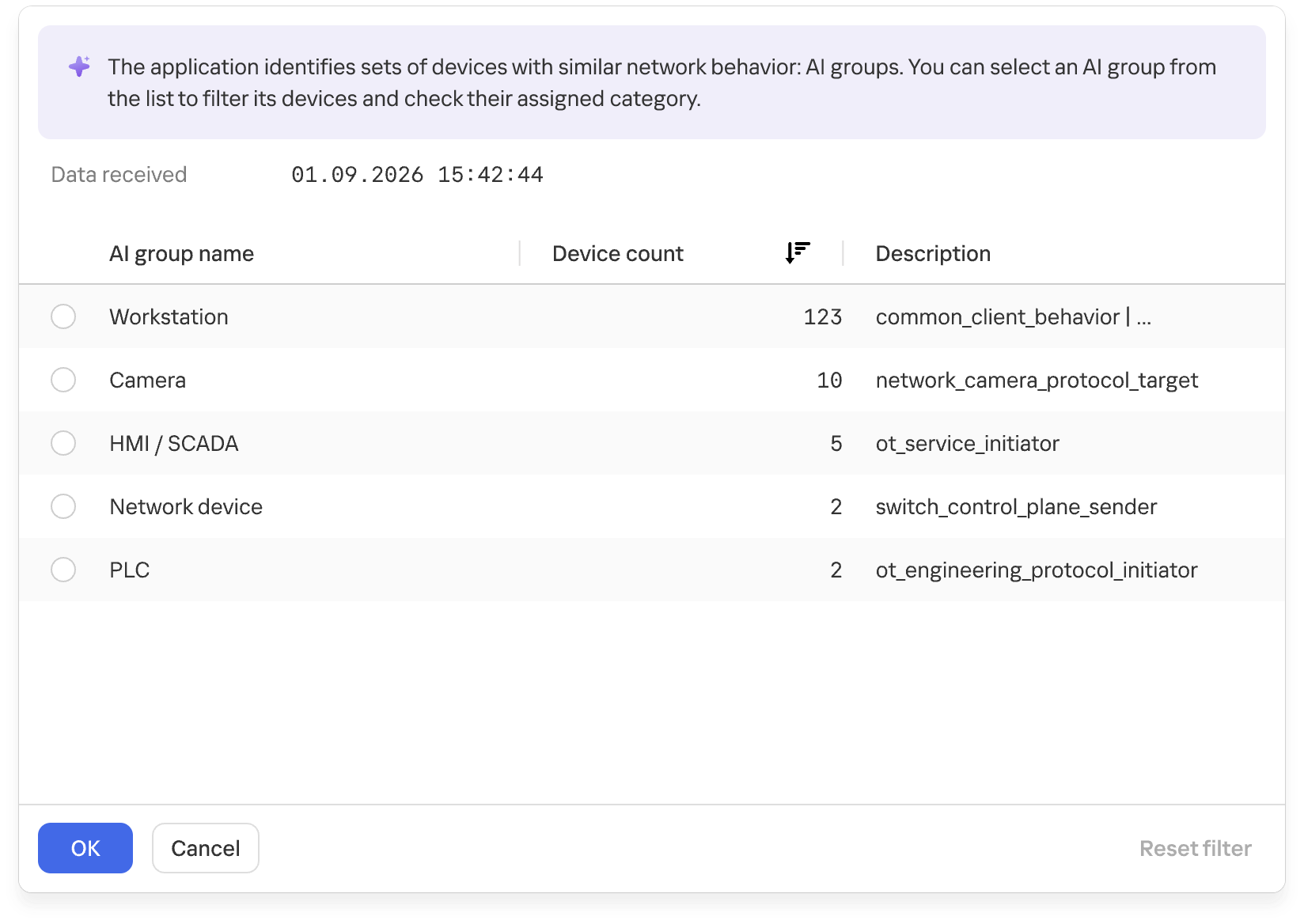
- For categorization, MLEP uses attention heads and monitors that identify common behavior across different assets and group devices accordingly. MLEP then takes information from Asset Discovery about the known categories of some assets and extends those categories to other assets in the same group. Because a device can show different types of activity, it may land in several groups. MLEP then makes a weighted assessment across all relevant groups.
Groups of devices with similar network behavior
At the final stage, the system verifies that assigning the category to the asset is permissible. This is again done by special rule monitors loaded into the NSN at system startup. The rules rely on asset metadata available from Asset Discovery and APMs.
- MLEP takes a similar approach to anomaly detection: an attention head and a monitor define an anomaly scenario, often loosely. When a monitor activates on such a scenario, MLEP generates an alert about unusual behavior.
The current version of MLEP ships with preconfigured heads and monitors.
The functional dynamic diagram below shows how events from devices on an industrial network are processed.
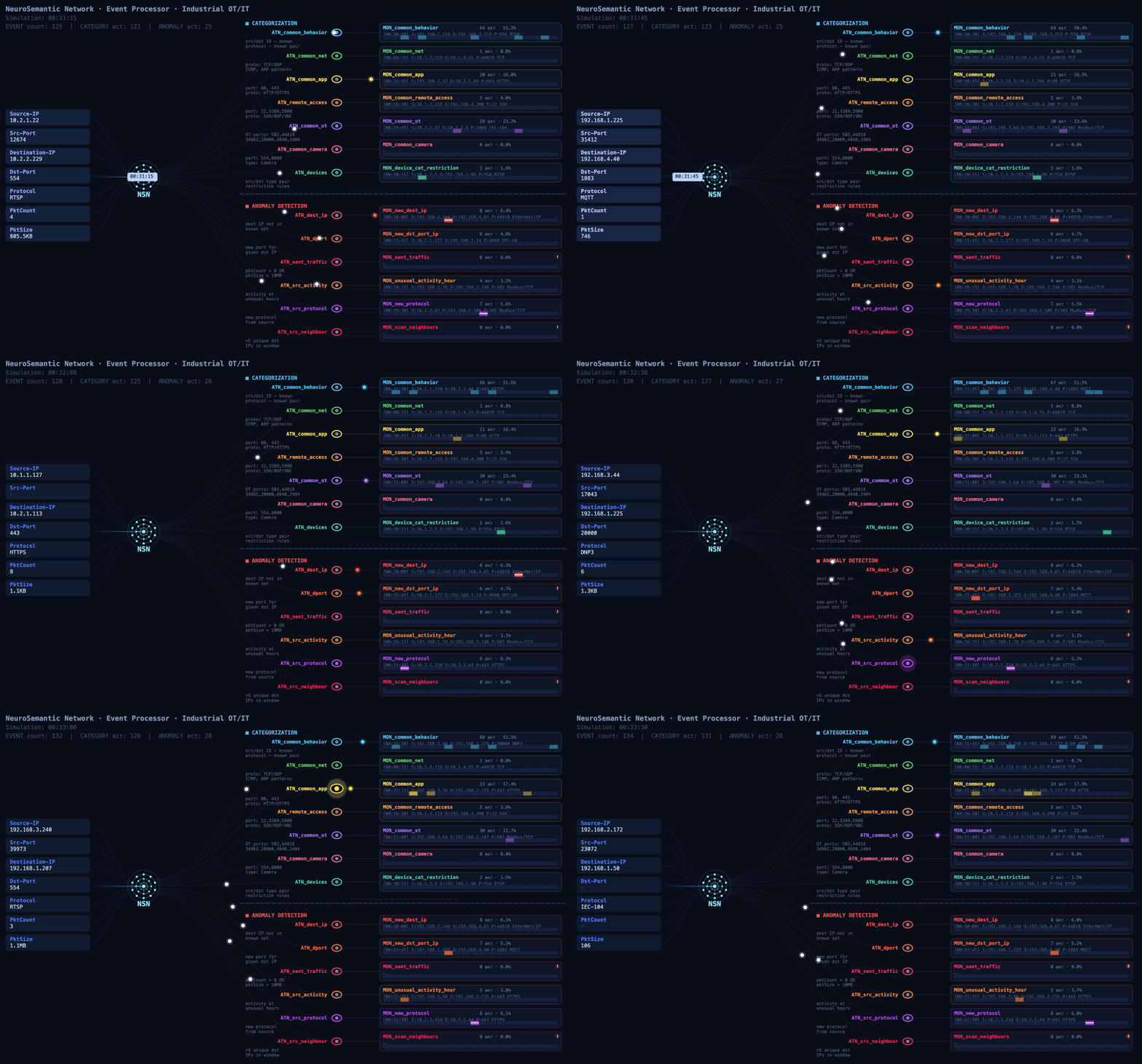
Event processing flow (click to play)
MLEP in practice: how behavior helps complete the asset inventory
At a facility with several similar production lines, device information may be more complete on some lines than on others. On one line, devices are identified as PLCs, while on another, after an upgrade, some hosts show up only as addresses: the available traffic didn’t provide enough information to determine their category. Still, these devices communicate with the same types of HMIs and process data collection servers. Their communication directions, frequency, and volumes may be similar.
That’s where MLEP comes in. It takes the categories of already known assets and matches recurring features of their network behavior against those of uncategorized devices. When the observed interactions turn out to be similar, MLEP can add a category for that host to the inventory.
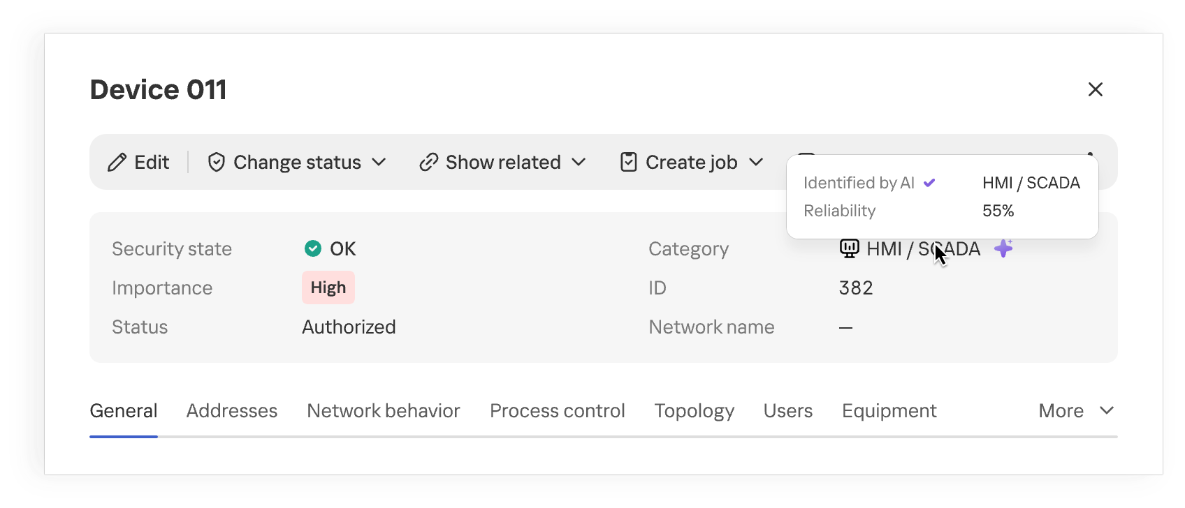
Device category suggested by MLEP
Once the category is refined, the industrial network map provides more context about the equipment on the network. When analyzing network activity, the analyst immediately sees the device’s suggested category and can skip looking up each IP address in the design diagrams. This approach is especially useful where equipment changes faster than the documentation is updated.
The suggested category is also checked against existing device information and defined constraints. This helps filter out some contradictory options, but prediction quality still depends on how much of the traffic is visible, especially if the device communicates only rarely.
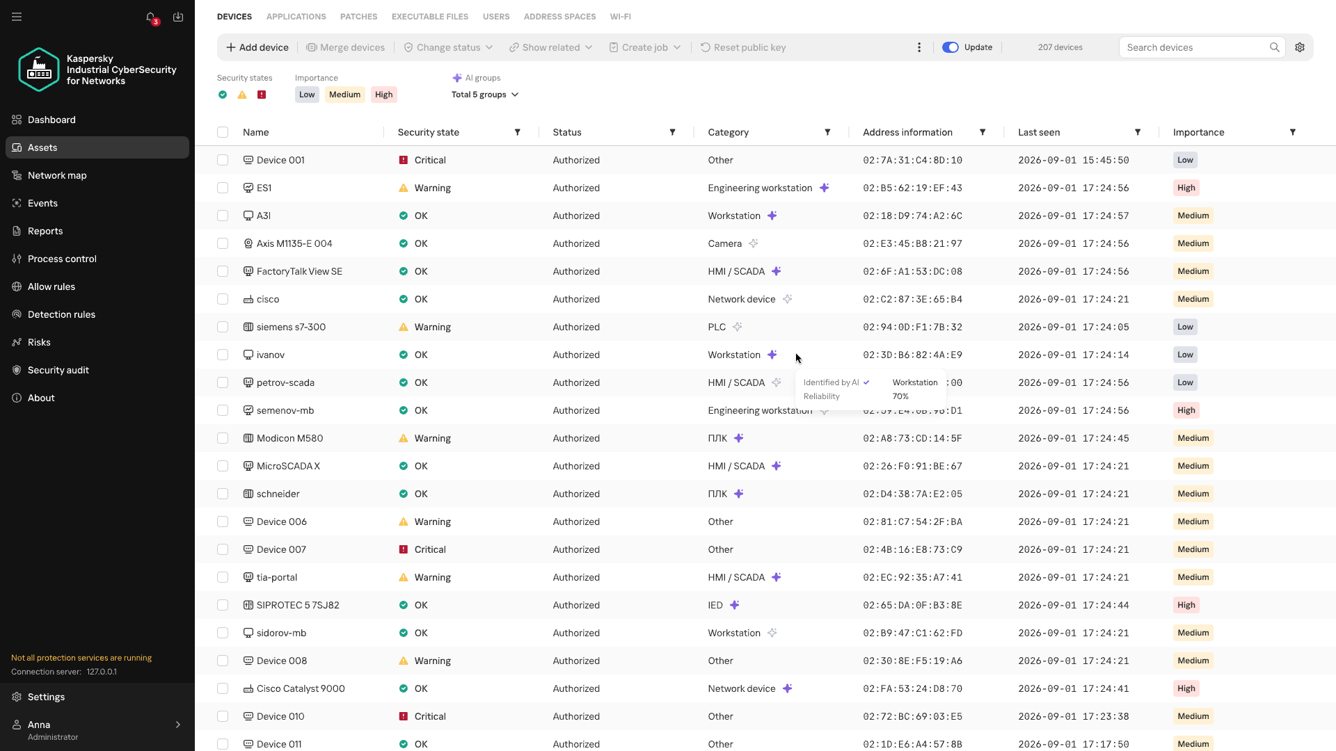
Anomalous activity and streaming statistics
Investigations of real-world attacks show that attackers actively use both standard tools and permitted protocols. You don’t always need to know an attacker’s specific technique in advance to spot potentially malicious activity. Signature-based detection helps find known signs of an attack, but it doesn’t assess how typical an observed interaction is for a particular device. MLEP compares current activity with the device’s usual network profile: which hosts it communicates with, which protocols it uses, when and how much data it transmits, its average packet size, and so on. The changes it detects help guide the direction of the investigation. Correlating these changes with other events and the operational context helps determine whether malicious actions could be behind them. When investigating an incident that has already been detected, anomalies help reconstruct the sequence of actions.
The first version of MLEP comes with six preconfigured monitors, one for each type of deviation from the device’s usual network profile:
| Anomaly | How it helps with event analysis |
| New external host | Flags a new external connection that wasn’t previously seen in the device’s observed behavior, even if the IP address isn’t listed among known IoCs. Helps check whether this connection appeared at the same time as other suspicious events. |
| New combination of destination address and port | Shows that the device has begun using a service it hasn’t used before. Once an incident has been detected, this helps trace new connections after the more critical events have been analyzed. |
| Unusually large volume of data sent | Highlights data transfers that are atypical for the device and helps correlate their timing and direction with other events. |
| Atypical activity time | Shows that the device was active at a time that’s unusual for it. In an already detected incident, this helps reconstruct the timeline of actions around the main alert. |
| New protocol | Helps spot a new method of communication, even when the device is communicating with familiar hosts. |
| Activity with signs of scanning | Shows that the device has started contacting an unusually large number of neighboring hosts. This signal helps reveal possible reconnaissance ahead of attempts to access equipment. |
During an investigation, anomalies help reconstruct the sequence of changes: when a specific host established new connections, switched protocols, increased its data transfer volume, or shifted its operating hours. Matching events by device and time shows an analyst how activity unfolded around an incident that has already been detected.
This is especially useful when some of the attacker’s actions fell outside the monitored scope or didn’t trigger other KICS technologies. Correlating these changes with the device’s role, protocol analysis data, and events from other technologies gives the analyst a more complete timeline. Behavioral anomalies show exactly where to look for the missing links and which network interactions need attention.
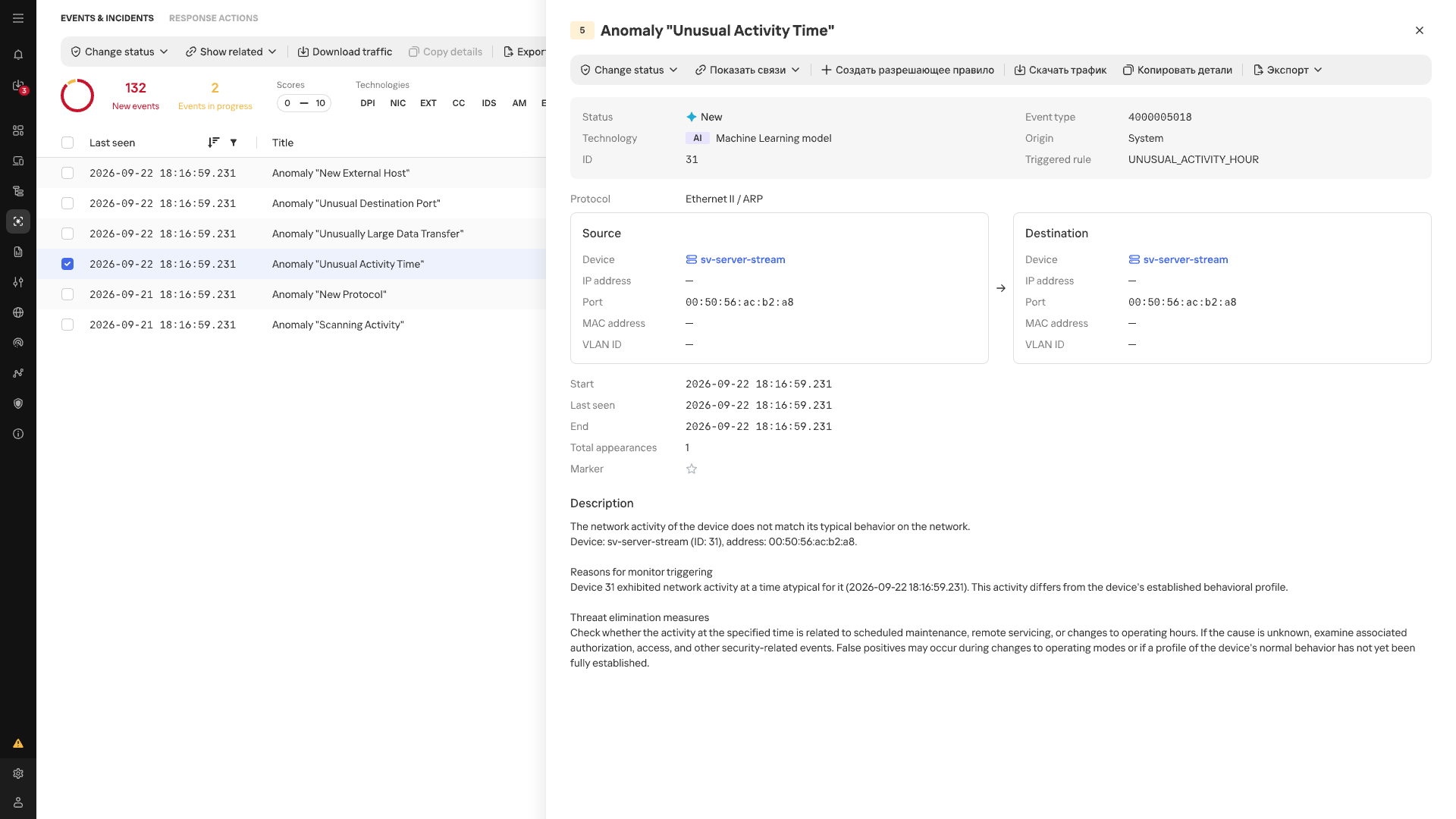
Atypical Activity Time anomaly card
In the event list, anomalies detected by MLEP are marked with an AI label. Each event shows its name, source, destination, timestamp, and the ID of the triggered scenario.
Conclusion
In an industrial network, whether behavior is anomalous depends on the host where it occurs and that host’s place in the industrial process. The repetitive nature of many communications makes a change in normal data exchange easier to spot, while knowing a device’s function and criticality helps gauge the possible consequences. Taken together, these observations make network traffic more than a list of connections: it helps assess new events in the context of a specific facility, even without an attack scenario known in advance. Machine learning technologies are well suited to this kind of comprehensive analysis, as they can process and organize huge streams of heterogeneous data. Starting with version 5.0, Kaspersky Industrial CyberSecurity for Networks handles this function with MLEP, which works effectively alongside the product’s existing functionality.